Recently, I’ve started a journey to “understand how LLMs work”.
Implementing something is a good way to understand it, so I’ve started the llm-runner project.
To start this project, it was natural to start with the architecture described in the fundamental paper Attention is all you need Vaswani et al., 2017.
In this post, we will focus on the general mathematical operations performed by LLMs, and their implementation in Rust. This post and the next one accompany the first PR on the llm-runner repository.
In the next post, we’ll see how we parse an actual model and make a program that runs it on user-written prompts.
What is a LLM?
LLMs can be seen as mathematical functions that transform sequences of tokens into a probability distribution over the token space. That is to say a function
$$\mathrm{llm}: T^{\mathrm{seq\_len}} \rightarrow [0, 1]^{n_T}$$where $T$ is the token space, $\mathrm{seq\_len}$ is the length of the sequence and $n_T$ is the size of the token space.
In Rust this would be written like this
fn llm(tokens: &[Token]) -> Vec<f32> {
    // ...
}
Given a sequence of tokens, an LLM can be used iteratively to generate the next token in the sequence, in a process called “Inference”.
This would for example look like
fn infer(tokens: &mut Vec<Token>, n: usize) {
    for _ in 0..n {
        let output = llm(tokens.as_slice());

        // Alternatively, sample output as a probability distribution.
        let argmax = output.iter().enumerate().max_by_key(|(_, &x)| x).unwrap().0;
        tokens.push(Token::from_token_id(argmax));
    }
}
How is the output of the LLM defined?
The mathematical operations performed by the LLM are determined by two components:
- The architecture of the LLM, which defines the operations that are successively applied to the input.
- The weights of the LLM, which are the parameters of these mathematical operations.
Here we will focus on the architecture described in Vaswani et al., 2017. This paper introduces the Transformer architecture, which leverages the attention mechanism—that is, the use of this operation:
$$\mathrm{Attention(Q, K, V)} = \mathrm{softmax}\left(\frac{QK^T}{\sqrt{d_k}}\right)V$$Where $Q$, $K$, and $V$ are the query, key, and value matrices. For now we ignore multi-head attention and work with a single head, so $d_k = d_{\mathrm{model}}$ and $Q$, $K$, and $V$ each lie in $\mathbb{R}^{\mathrm{seq\_len} \times d_{\mathrm{model}}}$. $\mathrm{softmax}$ is the softmax function.
The output of the attention operation is a matrix in $\mathbb{R}^{\mathrm{seq\_len} \times d_{\mathrm{model}}}$ whose rows are a contextualized representation of the input sequence: each position aggregates information from the whole sequence according to the attention weights.
Each row of the query matrix $Q$ is the vector at that position that encodes what information it seeks from the rest of the sequence.
Each row of the key matrix $K$ is the vector that pairs with queries to score compatibility between positions; together, $Q$ and $K$ determine how strongly each position attends to every position in the sequence (including itself).
Each row of the value matrix $V$ is the vector whose content is mixed into the output when that position is attended to.
The $\mathrm{softmax}$ function maps the raw scores to a probability distribution over the positions.
$$\mathrm{softmax}(x) = \frac{\exp(x)}{\sum_{i=1}^{n}\exp(x_i)}$$fn softmax(x: &[f32]) -> Vec<f32> {
// Directly translating the above formula would lead to computing exponential of large
// numbers, leading to numeric instability (esp on `f32`s).
// This implementation is mathematically equivalent, but more stable.
let max = x.iter().copied().fold(f32::NEG_INFINITY, f32::max);
let sum: f32 = x.iter().map(|&xi| (xi - max).exp()).sum();
x.iter().map(|&xi| (xi - max).exp() / sum).collect()
}
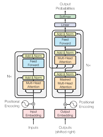
The Transformer model architecture as given in Vas17.
This schema describes the architecture of a Transformer model. It is composed of two stacks: an encoder and a decoder.
The encoder is responsible for encoding the input sequence into a sequence of hidden states. It can be seen as a function
$$\mathrm{encoder}: T^{\mathrm{seq\_len}} \rightarrow H^{\mathrm{seq\_len}}$$Where $H=\mathbb{R}^{d_{\mathrm{model}}}$ is the hidden state space of dimension $d_{\mathrm{model}}$. Vectors in $H$ embed a contextualized representation of the input sequence in a space of dimension $d_{\mathrm{model}}$.
The decoder is responsible for generating the output sequence from the hidden states. It can be seen as a function
$$\mathrm{decoder}: H^{\mathrm{seq\_len}} \times T^{n_{\mathrm{out}}} \rightarrow [0, 1]^{n_T}$$That will use the output of the encoder and the tokens of the output sequence so far to generate the next token in the sequence.
Embeddings
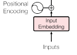
The embedding layer as given in Vas17.
In reality, the elements of the input and output sequences are not manipulated as discrete tokens inside the model, but as vectors in a real embedding space $\mathbb{R}^{d_{\mathrm{model}}}$ where $d_{\mathrm{model}}$ is a fixed constant for the model, typically much smaller than the vocabulary size $n_T$.
A sequence of length $\mathrm{seq\_len}$ is therefore represented as a matrix in $\mathbb{R}^{\mathrm{seq\_len} \times d_{\mathrm{model}}}$: one $d_{\mathrm{model}}$-dimensional row per position. The embedding layer maps a sequence of token indices to such a matrix.
In practice, the sequence of tokens of length $\leq \mathrm{seq\_len}$ is represented as a vector $x \in \{0,\ldots,n_T-1\}^{\mathrm{seq\_len}}$ with $x_i$ the id of the token at position $i$.
The embedding is then computed as follows: Let $W_e \in \mathbb{R}^{n_T \times d_{\mathrm{model}}}$ be the learnt token embedding matrix (row $j$ is the vector for token $j$) and let $P_e \in \mathbb{R}^{\mathrm{seq\_len} \times d_{\mathrm{model}}}$ be the matrix of positional encodings for those positions (fixed or learnt), so that each row encodes where the token sits in the sequence.
Then
$$\mathrm{embedding}: \{0,\ldots,n_T-1\}^{\mathrm{seq\_len}} \rightarrow \mathbb{R}^{\mathrm{seq\_len} \times d_{\mathrm{model}}}$$$$\mathrm{embedding}(x) = \mathrm{LayerNorm}(M(x)) \quad\text{where}\quad M(x)_{i,:} = (W_e)_{x_i,:} + (P_e)_{i,:}$$and $\mathrm{LayerNorm}$ is applied row-wise to $M(x)$.
$\mathrm{LayerNorm}$ is layer normalization along the feature dimension of each row; see here and the Rust code below for the definition.
src/layers/embeddings.rs:
//! Embeddings layer

use crate::{
    Error,
    layers::{Matrix, Norm},
};

use nalgebra::DMatrix;

pub struct Embeddings {
    pub norm: Norm,
    pub positions: Matrix,
    pub words: Matrix,
}

impl Embeddings {
    pub fn embed(&self, input: &[u32]) -> Result<DMatrix<f32>, Error> {
        let [vocab_size, d_model] = self.words.shape();

        let mut embeddings = DMatrix::zeros(input.len(), d_model);

        for (i, token) in input.iter().enumerate() {
            let t_id = *token as usize;
            if t_id >= vocab_size {
                return Err(Error::InconsistentShape);
            }

            embeddings
                .row_mut(i)
                .copy_from(&(self.words.row(t_id) + self.positions.row(i)));
        }

        self.norm.normalize_rows(&mut embeddings)?;

        Ok(embeddings)
    }
}
src/layers/norm.rs:
use crate::{Error, layers::Vector};

use {
    nalgebra::{DMatrix, DVector, DVectorViewMut},
    safetensors::tensor::TensorView,
};

pub struct Norm {
    bias: Vector,
    weight: Vector,
    epsilon: f32,
}

impl Norm {
    pub fn shape(&self) -> usize {
        self.bias.len()
    }

    pub fn normalize_row(&self, row: &mut DVectorViewMut<f32>) -> Result<(), Error> {
        let n = row.len();
        if n != self.shape() {
            return Err(Error::InconsistentShape);
        }

        let mean = row.mean();
        let inv_std = 1.0 / (row.variance() + self.epsilon).sqrt();

        *row -= &DVector::from_element(n, mean);

        *row *= inv_std;

        row.component_mul_assign(&self.weight);

        *row += &*self.bias;

        Ok(())
    }

    pub fn normalize_rows(&self, rows: &mut DMatrix<f32>) -> Result<(), Error> {
        let (nrows, n_cols) = rows.shape();

        if n_cols != self.shape() {
            return Err(Error::InconsistentShape);
        }

        let mut buf = vec![0.0f32; n_cols];
        for i in 0..nrows {
            for j in 0..n_cols {
                buf[j] = rows[(i, j)];
            }
            let mut view = DVectorViewMut::from_slice(&mut buf, n_cols);
            self.normalize_row(&mut view)?;
            for j in 0..n_cols {
                rows[(i, j)] = buf[j];
            }
        }
        Ok(())
    }
}
The Encoder Stack
The encoder is a stack of $N$ identical layers applied one after another. Each layer is a fixed pattern:
- First a multi-head self-attention block that computes how every position attends to every position
- Then, a position-wise feed-forward network (FFN) that further refines each position’s vector on its own: it takes the representation that attention has already contextualized and processes it in place, enriching what that slot encodes without pulling in information from other positions.
Writing $X \in \mathbb{R}^{\mathrm{seq\_len} \times d_{\mathrm{model}}}$ for the layer input, one encoder layer (in the post-norm style of [Vas17]) looks like
$$ \begin{aligned} X' &= \mathrm{LayerNorm}\bigl(X + \mathrm{MultiHead}(X)\bigr) \\ X'' &= \mathrm{LayerNorm}\bigl(X' + \mathrm{FFN}(X')\bigr)\,. \end{aligned} $$The fact that $X$ is added to the output of the attention block and $X'$ is added to the output of the FFN block is referred to as residual connections and represented by arrows that skip the Attention/FFN blocks.
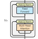
The encoder stack as given in Vas17. The input is forwarded to a multi-head attention block and an FFN block; each sublayer’s output is added to a residual and then normalized.
Multi-head attention
The single-head picture from earlier uses $d_k = d_{\mathrm{model}}$. In practice the model splits that width into several heads so it can attend in different representation subspaces in parallel.
Let $h$ be the number of heads. For each head $i$, the same sequence $X$ is mapped into that head’s queries, keys, and values by an affine map (matrix multiply plus bias, the bias broadcast to every row of $X$):
$$ Q_i = X W_i^Q + b_i^Q,\quad K_i = X W_i^K + b_i^K,\quad V_i = X W_i^V + b_i^V\,. $$The $W_i^Q, W_i^K, W_i^V$ and $b_i^Q, b_i^K, b_i^V$ are learned weights and biases specific to each head of each attention layer.
The shapes of $W_i^Q, W_i^K, W_i^V$ and $b_i^Q, b_i^K, b_i^V$ match $X \in \mathbb{R}^{\mathrm{seq\_len} \times d_{\mathrm{model}}}$ so that $Q_i$ and $K_i$ have $d_k$ columns and $V_i$ has $d_v$ columns. The output of one head is then the usual attention:
$$ \mathrm{head}_i = \mathrm{Attention}(Q_i, K_i, V_i)\,. $$The heads are then concatenated and mapped back to $d_{\mathrm{model}}$ with another affine map:
$$ \mathrm{MultiHead}(X) = \mathrm{Concat}(\mathrm{head}_1, \ldots, \mathrm{head}_h)\, W^O + b^O\,. $$Where $W^O$ and $b^O$ are learned weights and bias specific to each attention layer.
src/layers/attention.rs (linear and add_bias_rows live in src/layers/mod.rs):
//! Attention layer

use crate::{
    Error,
    layers::{Matrix, Vector, add_bias_rows, linear},
};

use {nalgebra::DMatrix, safetensors::tensor::TensorView};

pub struct Attention {
    pub q_weights: Matrix,
    pub q_bias: Vector,
    pub k_weights: Matrix,
    pub k_bias: Vector,
    pub v_weights: Matrix,
    pub v_bias: Vector,
    pub out_weights: Matrix,
    pub out_bias: Vector,
}

impl Attention {
    pub fn forward_multi_headed(
        &self,
        x: DMatrix<f32>,
        n_heads: usize,
    ) -> Result<DMatrix<f32>, Error> {
        let (seq, d_model) = x.shape();
        if d_model != self.q_weights.shape()[1] {
            return Err(Error::InconsistentShape);
        }
        if n_heads == 0 || d_model % n_heads != 0 {
            return Err(Error::InconsistentShape);
        }
        let d_head = d_model / n_heads;
        let scale = 1.0 / (d_head as f32).sqrt();

        let q = linear(&x, &self.q_weights, &self.q_bias);
        let k = linear(&x, &self.k_weights, &self.k_bias);
        let v = linear(&x, &self.v_weights, &self.v_bias);

        let mut attended = DMatrix::zeros(seq, d_model);
        for h in 0..n_heads {
            let c0 = h * d_head;
            let qh = q.view((0, c0), (seq, d_head));
            let kh = k.view((0, c0), (seq, d_head));
            let vh = v.view((0, c0), (seq, d_head));

            let mut scores = &qh * &kh.transpose();
            scores.scale_mut(scale);

            // Apply softmax transformation on each row of the scores matrix.
            softmax_rows(&mut scores);

            let ctx = &scores * &vh;
            attended.view_mut((0, c0), (seq, d_head)).copy_from(&ctx);
        }

        let mut out = attended * self.out_weights.transpose();
        add_bias_rows(&mut out, &self.out_bias);
        Ok(out)
    }
}
Feed-Forward Network
The FFN is a two-layer MLP that is applied row-wise to the input.
$$ \mathrm{FFN}(X) = \mathrm{GeLU}(X W_1 + b_1) W_2 + b_2\,. $$Where $W_1, W_2$ and $b_1, b_2$ are learned weights and biases specific to the FFN.
$\mathrm{GeLU}$ is the Gaussian Error Linear Unit function:
$$ \mathrm{GeLU}(x) = 0.5 x (1 + \mathrm{erf}(x / \sqrt{2}))\,. $$(The original Transformer FFN in [Vas17] uses $\mathrm{ReLU}$; models such as BERT and DistilBERT use $\mathrm{GeLU}$ instead. The formula above is the exact $\mathrm{GeLU}$ definition; the Rust snippet below uses the usual tanh-based approximation to it.)
src/layers/ffn.rs (apply_gelu is imported from src/layers/mod.rs):
//! Feed-forward network layer

use crate::{
    Error,
    layers::{Matrix, Vector, add_bias_rows, apply_gelu},
};

use {nalgebra::DMatrix, safetensors::tensor::TensorView};

pub struct Ffn {
    pub linear_1: Matrix,
    pub linear_2: Matrix,
    pub bias_1: Vector,
    pub bias_2: Vector,
}


impl Ffn {
    pub fn forward(&self, x: DMatrix<f32>) -> Result<DMatrix<f32>, Error> {
        let (_, n_cols) = x.shape();
        if n_cols != self.linear_1.shape()[1] {
            return Err(Error::InconsistentShape);
        }

        let mut y = x * self.linear_1.transpose();
        add_bias_rows(&mut y, &self.bias_1);
        apply_gelu(&mut y);

        let mut z = y * self.linear_2.transpose();
        add_bias_rows(&mut z, &self.bias_2);

        Ok(z)
    }
}
Projecting the Encoder’s output to the vocabulary
The output of the last layer of the encoder is a matrix in $\mathbb{R}^{\mathrm{seq\_len} \times d_{\mathrm{model}}}$ that is then projected to the vocabulary space.
$$ \mathrm{Project}(X) = X W + b\,. $$Where $W$ and $b$ are learned weights and bias specific to the projection layer.
The output of the projection layer is a matrix in $\mathbb{R}^{\mathrm{seq\_len} \times n_T}$ whose entries are the logits (a.k.a. unnormalized probabilities) for the next token.
Putting it all together
We can now put all these pieces together to implement a function that evaluates the output of an encoder-only model such as BERT.
Here is the final structure and evaluation function for the DistilBERT model: In the next post, we will parse an actual model to fill all the values in the structure and make a program that runs it on user-written prompts.
src/distilbert/structs.rs:
//! Structures for the DistilBERT model.

use crate::{
    Error,
    layers::{Attention, Embeddings, Ffn, Matrix, Norm, Vector, apply_gelu, linear},
};

use nalgebra::DMatrix;

pub struct DistilBert {
    pub embeddings: Embeddings,
    pub encoder: Vec<Stack>,
    pub vocab_layer: VocabLayer,
    pub d_model: usize,
    pub seq_len: usize,
    pub vocab_size: usize,
    pub n_heads: usize,
}

pub struct Stack {
    pub attention: Attention,
    pub attention_norm: Norm,
    pub ffn: Ffn,
    pub output_norm: Norm,
}

pub struct VocabLayer {
    pub norm: Norm,
    pub transform: Matrix,
    pub transform_bias: Vector,
    pub project: Matrix,
    pub project_bias: Vector,
}

impl DistilBert {
    pub fn evaluate(&self, input: &[u32]) -> Result<DMatrix<f32>, Error> {
        let mut output = self.embeddings.embed(input)?;
        for stack in &self.encoder {
            // TransformerBlock: sa_layer_norm(attn(x) + x), then output_layer_norm(ffn(h) + h)
            let residual = output.clone();
            let attn_out = stack.attention.forward_multi_headed(output, self.n_heads)?;
            let mut h = attn_out + residual;
            stack.attention_norm.normalize_rows(&mut h)?;

            let residual = h.clone();
            let ffn_out = stack.ffn.forward(h)?;
            let mut h = ffn_out + residual;
            stack.output_norm.normalize_rows(&mut h)?;
            output = h;
        }

        // DistilBertForMaskedLM: transform → activation → vocab_layer_norm → projector
        let mut h = linear(
            &output,
            &self.vocab_layer.transform,
            &self.vocab_layer.transform_bias,
        );
        apply_gelu(&mut h);
        self.vocab_layer.norm.normalize_rows(&mut h)?;
        let logits = linear(
            &h,
            &self.vocab_layer.project,
            &self.vocab_layer.project_bias,
        );

        Ok(logits)
    }
}